Sandbox
This section briefly describes how to use the sandbox either from a Python shell or via the REDHAWK IDE; a more detailed description is available in the Sandbox chapter.
Python Sandbox
The sandbox can be accessed directly from the command line and is used to manipulate new components and waveforms. This provides a very powerful means of testing and scripting tests for REDHAWK systems.
Open a Python session and import the sandbox:
>>> from ossie.utils import sbRunning a component
To get a list of available components, type:
>>> sb.catalog()
['rh.HardLimit', 'rh.SigGen', ...]
The displayed list is derived by scanning
$SDRROOT.HardLimitandSigGenare examples of existing components.Create the component object by typing:
>>> hardLimit = sb.launch("rh.HardLimit")
>>> sigGen = sb.launch("rh.SigGen")
After the constructor is finished, the components run as their own processes. If an absolute file path for a component’s Software Package Descriptor (SPD) file (
<component.spd.xml) is given as a constructor argument for the component instance, then that component is started irrespective of whether or not it is present in$SDRROOT.
Support widgets are available in the sandbox to help the developer interact with running components. There are a variety of widgets, including data sources and sinks, a speaker interface, and plotters. In this example, the plot widget is used.
To use plotting, the path to the eclipse directory of the installed IDE must be specified in the sandbox (this can also be done by setting the
RH_IDEenvironment variable to the absolute path of the Eclipse directory prior to starting the Python session):>>> sb.IDELocation("/path/to/ide/eclipse") >>> plot = sb.Plot()Create two plot objects by instantiating the
Plotclass twice and assigning the objects to local variables:>>> plot1 = sb.Plot() >>> plot2 = sb.Plot()
Connect the components together and connect the plots. The
connect()method tries to match the port; ambiguities can be resolved with the parametersusesPortNameandprovidesPortName. Connecting the plots to the components displays the Plot Application window.>>> sigGen.connect(hardLimit) >>> sigGen.connect(plot1) >>> hardLimit.connect(plot2)In this tutorial, the
SigGencomponent is configured before it is started to get a better visual. Set the frequency of theSigGenComponent equal to 5006:>>> sigGen.frequency = 5006Start everything in the sandbox:
>>> sb.start()The property values can now be set on the
HardLimitcomponent. The plot reflects the property change:>>> hardLimit.upper_limit = .8To inspect the properties and input/output ports of a component, invoke the component’s
api()method:>>> sigGen.api()To clean up, type
Ctrl+Dto end the Python session. The Python sandbox releases all components and cleans up whatever plots or additional widgets were created during the session.
The IDE Sandbox
This section provides an overview of how to use the sandbox in the REDHAWK IDE. The IDE sandbox provides a graphical environment for launching, inspecting, and debugging components, devices, nodes, services, and waveforms. In addition, via the REDHAWK Console, you can use the Python-based sandbox API to interact with objects that are running within the IDE sandbox.
The following procedure provides an example of launching and interacting with a component in the sandbox in the REDHAWK IDE.
In the REDHAWK Explorer view:
Expand the Sandbox to expose the Chalkboard.
Double-click the Chalkboard.
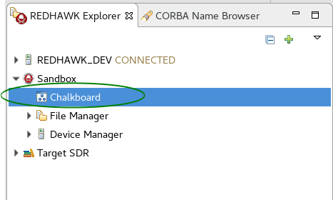
Open Chalkboard
From the Chalkboard:
Select the palette on the right; drag the
SigGen (cpp)component onto the Chalkboard. The component will initially be gray in color until launching is complete. When the component is finished loading, its background color is blue.SigGenwill be used to help test the newHardLimitcomponent.If the
SigGencomponent is not displayed, left-click therhfolder to display the list of available components.If the cpp implementation is not displayed, expand the list of implementations by left-clicking the arrow to the left of the component name and select the cpp implementation.
To zoom in and out on the diagram, press and hold Ctrl; then scroll up or down. Alternatively, press and hold Ctrl; then press + or -.
Right-click the
SigGencomponent, and select Start.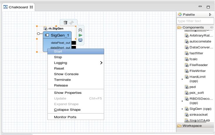
Start Component
Left-click the dataFloat_out port to select it, then right-click the port to open the port context menu, and select Plot Port Data.
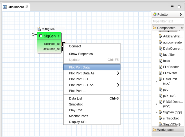
Plot Port Data
Open the Properties view and change the following signal properties:
- frequency: 100
- magnitude: 10
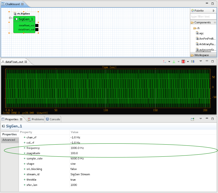
Change Property Value
Select the palette on the right, drag the
HardLimitcomponent onto the Chalkboard.Right-click the
HardLimitcomponent, click Start.Connect the dataFloat_out port on the
SigGencomponent to the dataFloat_in port on theHardLimitcomponent by clicking and dragging from the solid black output port to the input port.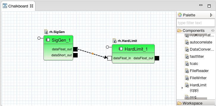
Connect Ports
Right-click the dataFloat_out port on the
HardLimitcomponent, click Plot Port DataNotice that the output has been hard limited by the
HardLimitcomponent